# Lectures on AdS/CMT ## Organization of the lectures These lectures are not intended to be formal in any sense, but instead to give an intuitive glimpse on the field of holographic methods applied to condensed matter systems. Formal proofs of many of the issues here discussed can be found in the literature, while some of them still under active investigation. The subject to be discussed are roughly the following: 1. Introduction: 1. Bottom-up approach: symmetry $+$ kinematics $=$ dynamics & thermodynamics 1. Revisiting QFTs 1. Definition via symmetries and field content 2. Definition at an UV fixed point 3. Path integral formula and response functions 2. Applying these ideas to holography 1. Reformulation of the above approach 2. The holographic formula and response functions 2. Superconductors 1. Why AdS/CMT: the problem of T$_c$ superconductors 1. Historic introduction 1. Low T$_c$ and BCS intuition 2. High T$_c$ and the isotopic effect 2. The High T$_c$ phase diagram 2. Holographic superconductors 1. Definition of the model 1. Application of the ideas of lecture 1. 2. Solution 1. Equations of motion 2. Boundary conditions 3. Critical temperature 4. Conductivity 3. Sophistications 1. Magnetic field 2. Doping 3. $p$ wave superconductor 2. Coleman-Mermin-Wagner 3. Metals 1. Fermi theory 2. Fermi surface 3. Quasiparticles 4. Holographic realization 1. Neutron star 2. Electron star 5. Sophistications 1. Chemical potential 2. Finite volume effects 2. Pomeranchuk instabilities 4. More advanced stuff 1. Nematic and chessboard phases 2. Flat bands 3. Crystals To keep anxiety under control, the lectures are organized in green, yellow and red zones, bellow the following marks :::success :white_check_mark: ::: In the green zone we find material to take away. This is the main line of developement of the course, and the issues explained are expected to be understood. :::warning :warning: ::: The yellow zone contains material which is not essential or lies outside of the main line of developement, even if it is covered as part of the basic physics courses. If you get lost under this sign, don't panic, this is just a disgression and you will be able to keep engaged with the main goals of the course. :::danger :red_circle: ::: The red zone is made of more advanced or recent material. This is included to make contact to some of the present research in the subject, and it is not closed nor complete in any sense. Getting lost here has to be expected. --- ## Lecture one: introduction > *What use is a newborn baby?* ### Bottom-up approach: symmetry $+$ kinematics $=$ dynamics & thermodynamics #### Revisiting QFTs How do we define a quantum field theory? 1. Symmetry: we start by choosing our symmetry group $G$. A subgroup $S\subset G$ corresponds to the *spacetime point symetries*, whose elements $s\in S$ map any point $x=(t,\vec x_d)$ of spacetime into a physically equivalent point $x'=s(x)$, leaving one point invariant. The complete group $G$ is usually written as a product of $S$ with an internal symmetries subgroup $I$ as $G=S\times I$. 2. Kinematics: next, we choose our fields $\Phi_{i \mu}(x)$ with $i\in \{1,\dots,d_R\}$ and $\mu\in\{1,\dots,d_\Sigma\}$, where $d_R$ is the dimension of a certain representation $R(I)$ of the internal symmetries, while where $d_\Sigma$ is the dimension of a representation $\Sigma(S)$ of the spacetime factor. Under the combined action of a spacetime transformation $s\in S$ and an internal one $g\in I$, the fields then transform according to $\Phi'_{i\mu}(x)=R_{ij}(g)\Sigma_{\mu\nu}(s)\,\Phi_{j\nu}\left(s^{-1}(x)\right)$ 3. Dynamics: finally, we write the most generic Lagrangian ${\cal L}_{\sf QFT}$ containing all the (renormalizable) terms invariant under the symmetries that can be constructed with our fields. Any ommited term is generated by renormalization. This Lagrangian is then used in a functional integral, in order to compute observables, according the the standard rules We define the generating functional $Z[{\cal J}]=\int \Pi_{i\mu} {\cal D}\Phi_{i\mu}e^{i \int d^{d+1}x \,\left({\cal L}_{\sf QFT}+{\cal J}_{i\mu}{\cal O}_{i\mu}\right)}$ And then calculate correlators of the operators ${\cal O}_{i\mu}$ by taking derivatives $\langle T\{{\cal O}_{i\mu}(x){\cal O}_{j\nu}(y)\dots\}\rangle=\left.\frac{i^n}{Z[{\cal J}]}\frac{\delta Z[{\cal J}]}{\delta {\cal J}_{i\mu}(x)\delta {\cal J}_{j\nu}(y)\dots}\right|_{{\cal J}_{i\mu}=0}$ 4. Thermodynamics: to describe a QFT in equilibrium at finite temperature, we go into Euclidean space using a Wick rotation $t\to i\tau$ and then compactify the Euclidean time $\tau=\tau+\beta$ in a circle of length $\beta=1/T$. The above formulas can be straigthforwardly adapted. > Examples: > > 1. Relativistic QFTs > If we choose the symmetry group $G$ as $G=S\times I$ with $S=SO(d,1)$, we are constructing a Lorentz invariant QFT. Notice that, even if translations are not part of the point symmetry group, the field theoretical construction results in a Poincaré invariant theory. This is completely general. > > 1. Scalar QFTs > We can now select the field content as a single scalar field, meaning a field that under Lorentz transformations transforms as $\phi'(x)=\phi(s^{-1}(x))$. > > The internal symmetries can be chosen in a buch of different ways, for example > > 1. When the group is $I=\mathbb{Z}_2$ then the scalar can be even or odd under it, meaning $\phi'(x)=\pm\phi(x)$. > > For the odd case $\phi'(x)=-\phi(x)$, the most generic lagrangian contains all the even powers of $\phi$ and its derivatives $\partial_\mu\phi$ with their indices contracted with the minkowskian metric $\eta^{\mu\nu}$. We then get a general function with the form ${\cal L(\eta^{\mu\nu}\partial_\mu\phi\partial_\nu\phi,\phi^2)}$ (whose higher power of $\phi$ is limited by renormalizability depending on the dimension). > > The even representation instead satisfies $\phi'(x)=\phi(x)$, then odd powers of $\phi$ and its derivatives are also allowed, and we have the result ${\cal L}_{\sf QFT}={\cal L(\eta^{\mu\nu}\partial_\mu\phi\partial_\nu\phi,\phi)}$. > > 2. Let us now replace the internal part by $I=U(1)$ > > If we put the scalar in the fundamental representation $\phi'(x)=e^{i\varphi}\phi(x)$ where $\varphi$ is the angle that defines a $U(1)$ rotation, then any term of the Lagrangian would have to be constructed from powers of $\eta^{\mu\nu}\partial_\mu\phi\partial_\nu\phi^*$ and $\phi \phi^*$, resulting in ${\cal L}_{\sf QFT}={\cal L(\eta^{\mu\nu}\partial_\mu\phi\partial_\nu\phi^*,\phi\phi^*)}$. > > 3. We can in principle choose a different internal symmetry group, like for example $O(3)$, and the generics of the construction remain the same. > > Putting the field in the fundamental representation $\phi'_a(x)=R_{ab}\phi_b(x)$ where $R_{ab}$ is a rotation matrix, then the lagrangian has o be constructed from $\eta^{\mu\nu}\delta_{ab}\partial_\mu\phi_a\partial_\nu\phi_b$ and $\delta_{ab}\phi_a\phi_b$ in the form ${\cal L}_{\sf QFT}={\cal L}(\eta^{\mu\nu}\delta_{ab}\partial_\mu\phi_a\partial_\nu\phi_b,\delta_{ab}\phi_a\phi_b)$ > 2. Vector QFTs > We can choose a different representation of the spatial symmetries, for example the vector one $A'_\mu(x)=\Lambda_\mu^{\,\nu} A_\nu(s^{-1}(x))$. > > With a trivial internal group $I=\{id\}$ we immediately get a (generalized) Proca model with the form ${\cal L}_{\sf QFT}={\cal L}(F_{\mu\nu}F^{\mu\nu},A_\mu A^{\mu})$ (similarly to the scalar case, the higher powers get limited if we impose renormalizability). > > 3. Spinor QFTs > A spinor QFT is constructed with a field in the spinorial representation of $SO(d,1)$ transforming as $\psi_\alpha=S(\Lambda)_{\alpha\beta}\,\psi_\beta$, its Lagrangian is a function of the invariants. Depending on the dimension, those are for example $\bar\psi\partial\!\!\!/\psi$ and $\bar\psi\psi$, and also $\eta^{\mu\nu}(\bar\psi\partial_\mu\psi)(\bar\psi\partial_\nu\psi)$, $\eta^{\mu\nu}(\bar\psi\gamma^5\gamma_\mu\psi)(\bar\psi\gamma^5\gamma_\nu\psi)$, $(\bar\psi\gamma^5\psi)^2$, etc. > > 4. Generic Lorentzian QFTs > To construct a QFT with more fields, we choose a reducible representation of $SO(d,1)$, with for example a vector and a certain number of scalars. > 4. Conformal QFTs > In this case, the spacetime symmetry group is chosen as the conformal group $SO(d,2)$ > 1. Conformal scalar: we can define the QFT in an conformally invariant point in three dimensions by choosing the scalar dimension as $\phi'(x)=\lambda^{-1}\phi(\lambda^{-1}x)$. > > For the $\mathbb{Z}_2$ internal symmetry case studied before, in any of their representation, we can write the most generic Lagrangian as > > ${\cal L}_{\sf QFT}=-\frac12\eta^{\mu\nu}\partial_\mu\phi\partial_\nu\phi+\frac14\alpha \,\phi^4$ > 2. Conformal vector: for a vector field theory with conformal symmetry in three dimensions, we define $A_\mu'(x)=A_{\mu}(\lambda^{-1}x)$. The only possible Lagrangian in three dimensions then reads ${\cal L}_{\sf QFT}=-\frac14F_{\mu\nu}F^{\mu\nu}$. > > 5. Galilean QFTs > Here we choose the Euclidean group $SO(3)$ as the (purely spatial) spacetime group $S$ > > 1. Scalar QFT > Lets choose our field content in the scalar representation of the Euclidean group $\phi'(x)=\phi(s^{-1}(x))$ > > With the internal group as $I=\mathbb{Z}_2$ as before, let us put the field in the odd representation. > > Since the time does not interfere with the space transformations, higher spatial derivatives can be included. The more generic Lagrangian then reads ${\cal L}_{\sf QFT}={\cal L}(\dot \phi^2,\delta^{ij}\nabla_i\phi\nabla_j\phi,(\nabla^2\phi)^2,\delta^{ij}\delta^{kl}\nabla_i\nabla_k\phi\nabla_j\nabla_l\phi,\dots,\phi)$ > 6. Scale invariant Galilean QFTs > These are theories with scale invariance under non symmetric scalings of space and time, for whcih $t'=\lambda^zt$ while $\vec x=\lambda \vec x$. > > 1. Scalar $z=3$ QFT > Lets choose again the scalar representation of the Euclidean group $\phi'(x)=\phi(s^{-1}(x))$ and the field scaling as $\phi'(x)=\phi(\lambda^{-1}x)$ in three space dimensions. We get > > ${\cal L}_{\sf QFT}=\frac12\dot\phi^2+L(\nabla^6,\phi)$ > > where $L(\nabla^6,\phi)$ represent a general combination of six derivatives with an arbitrary even powers of the scalar field. > > 7. Crystaline QFTs > The point spacetime group $S$ can be chosen as a discrete rotational group, of the kind realized in a crystaline lattice. This is useful to describe the physics of crystals, as for example fermions in graphene. An easy way to organize the construction of renormalizable QFTs, is to define the it by its symmetries at an ultraviolet fixed point (that is a point which is scale invariant, eventually conformally invariant), there constructing the corresponding Lagrangian, and later *deforming* it by adding UV irrelevant terms that breaks the scale symmetry. In this way, QFTs are organized by the fixed point around which they are defined, and the symmetries broken by the deformation. > Examples > In our example 2-1 above, we can deform out of the conformal point by adding the *mass* term $-\frac12m\phi^2$, which in turn generates by renormalization all even powers of $\phi$, ending up with the result of example 1-1-1. > > In our example 4-1, deforming the QFT by adding any power of the scalar field, moves it our of the scale invariant point into the Lagrangian of example 3-1. Then we can then rephrase the above construction as 1. Symmetry: we start by choosing our symmetry group $G$. A subgroup $S\subset G$ corresponds to the *spacetime point symetries*, whose elements $s\in S$ map any point $x$ of spacetime into a physically equivalent point $x'=s(x)$, leaving one point invariant. **We add some sort of scale invariance, to describe an ultraviolet fixed point**. The complete group $G$ is usually written as a product of $S$ with an internal symmetries subgroup $I$ as $G=S\times I$. 2. Kinematics: next, we choose our fields $\Phi_{i \mu}(\vec x)$ with $i\in \{1,\dots,d_R\}$ and $\mu\in\{1,\dots,d_\Sigma\}$, where $d_R$ is the dimension of a certain representation $R(I)$ of the internal symmetries, while where $d_\Sigma$ is the dimension of a representation $\Sigma(S)$ of the spacetime factor. **This includes choosing a scaling dimension $q$ for all the fields**. Under the combined action of a spacetime transformation $s\in S$ and an internal one $g\in I$, the fields then transform according to $\Phi'_{i\mu}(x)=R_{ij}(g)\Sigma_{\mu\nu}(s)\lambda^q\,\Phi_{j\nu}\left(\lambda^{-1}s^{-1}(x)\right)$ 3. Dynamics: finally, we write the most generic Lagrangian containing all the terms invariant under the symmetries that can be constructed with our fields, **and deform out of the fixed point by adding UV irrelevant terms that break scale invariance.** additional terms are then generated by renormalization. This Lagrangian is then used in a functional integral, in order to compute observables, according the the standard rules We define the generating functional $Z[{\cal J}]=\int \Pi_{i\mu} {\cal D}\Phi_{i\mu}e^{i \int d^{d+1}x \,\left({\cal L}_{\sf QFT}+{\cal J}_{i\mu}{\cal O}_{i\mu}\right)}$ And then calculate correlators of the operators ${\cal O}_{i\mu}$ by taking derivatives $\langle T\{{\cal O}_{i\mu}(x){\cal O}_{j\nu}(y)\dots\}\rangle=\left.\frac{i^n}{Z[{\cal J}]}\frac{\delta Z[{\cal J}]}{\delta {\cal J}_{i\mu}(x)\delta {\cal J}_{j\nu}(y)\dots}\right|_{{\cal J}_{i\mu}=0}$ 4. Thermodynamics: to describe a QFT in equilibrium at finite temperature, we go into Euclidean space using a Wick rotation $t\to i\tau$ and then compactify the Euclidean time $\tau=\tau+\beta$ in a circle of length $\beta=1/k_BT$. The above formulas can be straigthforwardly adapted. :::warning :warning: ::: For the step 3 of our construction, we need to know all the conformally invariant tensors with indices in the corresponding representations. A conformally invariant tensor is an object $T_{\mu_1\dots\mu_n\,a_1\dots a_m}$ that satisfies $T_{\mu_1\dots\mu_n\,a_1\dots a_m}=\left|\frac{\partial s(x)}{\partial x}\right|^{-1}\Sigma_{\mu_1\mu'_1}\dots\Sigma_{\mu_n\mu'_n}\,R_{a_1a'_1}\dots R_{a_ma'_m}\,T_{\mu_1'\dots\mu_n'\,a_1'\dots a_m'}$ Then an invariant term in the Lagrangian reads $T_{\mu_1\dots\mu_n\,i_1\dots i_m}\Phi_{i_1\mu_1}(x)\dots\Phi_{i_n\mu_m}(x)$ Notice that kinetic terms are included in the present discussion if we include among our fields $\Phi_{i\mu}(x)$ both the fundamental fields and their derivatives. In the above construction, higher derivative are in principle allowed, but one has to be careful to avoid higher *time* derivatives which would generically give rise to ghosts. > Examples > In the example 1-1 above, the only invariant tensor in the vector representation of $SO(2,1)$ that can be used to contract derivatives is the Minkowskian metric $\eta_{\mu\nu}$ and its products $\eta_{\mu\nu}\eta_{\rho\sigma}\dots$ > > Example 1-1-2 is understood by decomposing the $U(1)$ field as $\phi=\phi_1+i\phi_2$ and coupling the components $\phi_i$ by making use of the invariant tensor $\delta_{ij}$. > > In example 1-1-3 the invariant tensor of $O(3)$ with indices in the fundamental representation are built from $\delta_{ab}$ and its products > > The case of example 1-2 is similar to the derivatives of example 1-1, the only invariant tensor is the Lorentz metric and its products. > > For the spinors of example 1-3, the invariant tensor are constructed out products and contractions of the metric $\eta_{\mu\nu}$ and the Dirac matrices $\gamma^\mu_{\alpha\beta}$ and, depending on the dimension, the chiral matrix $\gamma^5_{\alpha\beta}$. > > In example 3 the only invariant tensor in the vector representation of $SO(3)$ is the Kronecker delta $\delta_{ab}$ and its products. :::success :white_check_mark: ::: One of the applications of the path integral formula that will be useful in the holographic context is the calculation of *"response functions"*, defined as the change in an expectation value when there is a change in a source. Assume we want to charatherize the change in $\langle{\cal O}_{i\mu}\rangle$ when the source ${\cal J}_{j\nu}$ is changed. Notice that this is not necessarily the source of the same operator. We can write $Z[{\cal J}]=\int \Pi_{i\mu} {\cal D}\Phi_{i\mu}e^{i \int d^{d+1}x \,\left({\cal L}_{\sf QFT}+{\cal J}_{i\mu}{\cal O}_{i\mu}+\delta{\cal J}_{j\nu}{\cal O}_{j\nu}\right)}$ Both sources are turned on. Taking the derivative of this expression with respect to ${\cal J}_{i\mu}$ and evaluating the result in ${\cal J}_{i\mu}=0$ give us, according to the above formula, the expectation value of ${\cal O}_{i\mu}$ in the presence of $\delta{\cal J}_{j\nu}$ $\langle {\cal O}_{i\mu}(x)+ \delta{\cal O}_{i\mu}(x)\rangle=\left.\frac{i}{Z[{\cal J}]}\frac{\delta Z[{\cal J}]}{\delta {\cal J}_{i\mu}(x) }\right|_{{\cal J}_{i\mu}=0}$ Since the source that we are changing $\delta{\cal J}_{j\nu}$ is infinitesimal, we can expand $Z[{\cal J}]=\int \Pi_{i\mu} {\cal D}\Phi_{i\mu}e^{i \int d^{d+1}x \,\left({\cal L}_{\sf QFT}+{\cal J}_{i\mu}{\cal O}_{i\mu}\right)}\left(1+\int d^{d+1}y\,\delta{\cal J}_{j\nu}(y){\cal O}_{j\nu}(y)\right)$ This allows us to write $\left\langle {\cal O}_{i\mu}(x)+ \delta{\cal O}_{i\mu}(x)\right\rangle=\left\langle T\left\{{\cal O}_{i\mu}(x)\left(1+\int d^{d+1}y\,\delta{\cal J}_{j\nu}(y){\cal O}_{j\nu}(y)\right)\right\}\right\rangle$ rearranging $\left\langle {\cal O}_{i\mu}(x)+ \delta{\cal O}_{i\mu}(x)\right\rangle=\left\langle{\cal O}_{i\mu}(x)\rangle+\int d^{d+1}y\,\delta{\cal J}_{j\nu}(y)\langle T\left\{{\cal O}_{j\nu}(y){\cal O}_{i\mu}(x)\right\}\right\rangle$ from which we get our response function $\frac{ \delta\langle{\cal O}_{i\mu}(x)\rangle}{\delta{\cal J}_{j\nu}(y)}=\langle T\left\{{\cal O}_{j\nu}(y){\cal O}_{i\mu}(x)\right\}\rangle$ This is known as the *"Kubo formula"*, and it is very useful in AdS/CMT. > Example: electric conductivity > > The electric conductivity is the response in the electric current when we change the electric field. The operator that couples to the electric current is the vector potential $\vec A$ (this plays the role of ${\cal J}_{i\mu}$, while the current plays the role of ${\cal O}_{i\mu}$). In the $A_0=0$ gauge in Fourier space, a small elecric field is given by $\delta\vec E=-i\omega \,\delta\vec A$ (this plays the role of $\delta {\cal J}_{j\nu}$). This implies that the electric conductivity can be regarded as the change in the electric current when we change the vector potential. We then have > > $\sigma_{ij}(\omega, \vec x,\vec y)=\frac{\delta j_i(\omega,\vec x)}{\delta E_j(\omega,\vec y)}=\frac{1}{i\omega}\langle T\{j_i(\omega,\vec x)j_j(\omega,\vec y)\}\rangle$ > > Similar calculations give us expressions for the magnetic susceptibility, the thermal conductivity, the elasticity moduli, the viscosity, etc. #### Aplying these ideas to holography Now we want to adapt theses ideas to construct, instead of a Lagrangian QFT to be treated perturbatively in a functional integral, an holographic description of a strongly coupled QFT. In other words, we aim to start with the symmetries and the field content, adding up an additional dimension, to end up with a higher dimensional dual that correctly includes them. First lets face step 1: symmetries. We need to start with a relativistic or Galilean theory with scale invariance, or in other words with a conformal (example 2) or a Lifshitz (example 4) theory (the crystaline case of example 5 could also be considered, but it leads to some subtleties that we want to ommit at this stage). Adding a holographic direction implies to enlarge the dimensions of spacetime by one, which rises the question of how to generalize the spacetime point symmetries. A natural solution is to promote it to an isometry of the higher dimensional manifold. In the conformal case, this is done by equiping it with an AdS metric $ds^2=L^2\left(\frac{dr^2}{r^2}+r^2(-dt^2+d\vec x_d^2)\right)$ whose isometries are known to correspond to $SO(2,d)$ In the Lifshitz case, we can put a metric with the form $ds^2=L^2\left(\frac{dr^2}{r^2}-r^{2z} L^{2(z-1)}dt^2+r^2d\vec x_d^2\right)$ which is invariant under the corresponding scalings and Euclidean transformations. In both cases, the "boundary" has a metric that reproduces the spacetime point symmetries of our QFT, and we can then state that it *"lives at the boundary"* of the bulk spacetime. Now, in extending the internal symmetry group $I$ to the bulk, one may naively impose that the bulk theory is invariant under the same group $I$ as the boundary QFT. However, this may result on a too strong imposition. Indeed, when a symmetry transformation $g\in I$ is made on the boundary, there is no need for *the same* transformation to be applied at any single point in the AdS interior. Instead, we can just apply a local transformation $g(x,r)$ whose boundary value is given by $g$. In other words, we are defining the bulk theory as a *gauge theory* whose gauge invariance group is $I$. A detail is that this can be done smootlhy only for continuous symmetries, the discrete part of $I$ is extended to the bulk as global symmetries. Notice that even if most of the gauge transformations correspond to redundacies on the definitions of the fields and are not considered to be physical, the global part of the gauge group, given by the large gauge trasnformations that are non-trivial at the boundary, still have a phisical content. This would be true for the internal factor $I$, but also for the spacetime point factor $S$. Gauging spacetime symmetries implies defining a gravitational theory in the bulk, invariant under general changes of coordinates. This theory needs to have an AdS or Lifshitz ground state. Then step 1 can be replaced by 1. Symmetry: we start by choosing our symmetry group $G$. A subgroup $S\subset G$ corresponds to the *spacetime point symetries*, whose elements $s\in S$ map any point $x$ of spacetime into a physically equivalent point $x'=s(x)$, leaving one point invariant. We add some sort of scale invariance, to describe an ultraviolet fixed point. We add one dimension, and in the resulting spacetime we define a gravitational theory with a ground state (AdS or Lifshitz) whose isometries reproduce the scale invariance. The complete group $G$ is usually written as a product of $S$ with an internal symmetries subgroup $I$ as $G=S\times I$. **The bulk theory has gauge invariance under the continuous part of $I$** Now we move into step 2: field content. We need to define the field content in the bulk theory, and the way those fields transform under the symmetries. :::warning :warning: ::: To get an intuition on how the field content can be chosen for the holographic dual of a given QFT, we can have a look to a well understood kind of duality: the electromagnetic one. We start with Maxwell's Lagrangian ${\cal L}=\frac1{4e^2} F^{\mu\nu}(A)F_{\mu\nu}(A)$ where $e$ is the electromagnetic coupling and $F_{\mu\nu}(A)=\partial_\mu A_\nu-\partial_\nu A_\mu$. Noticing that $\partial_\mu \tilde F^{\mu\nu}(A)=0$ whith $\tilde F_{\mu\nu}(A)= \epsilon_{\mu\nu}^{\;\;\;\rho\sigma}F_{\rho\sigma}(A)$ we can write ${\cal L}=\frac1{4e^2} F^{\mu\nu}(A)F_{\mu\nu}(A)+\frac1{\sqrt{2}}{\cal J}_\nu \,\partial_\mu \tilde F^{\mu\nu}(A)$ So we have coupled the system to an external current ${\cal J}_\nu$, with an operator that vanishes on shell. However, such adition of zero is not completly meaningless, since now we can forget that $F^{\mu\nu}(A)$ is a function of $A_\mu$. Indeed, if we replace the above action by ${\cal L}=\frac1{4e^2} F^{\mu\nu}F_{\mu\nu}+\frac1{\sqrt{2}}{\cal J}_\nu \,\partial_\mu \tilde F^{\mu\nu}$ where now $F_{\mu\nu}$ is undertood as a fundamental field, and now vary it with respect to ${\cal J}_\nu$, we obtain the equation of motion $\partial_\mu \tilde F^{\mu\nu}=0$ This "zero curl" equation is solved by introducing a potential $A_\mu$ and writing $F_{\mu\nu}=F_{\mu\nu}(A)=\partial_\mu A_\nu-\partial_\nu A_\mu$. Replacing back into the action, we get our original Maxwell's form ${\cal L}=\frac1{4e^2} F^{\mu\nu}(A)F_{\mu\nu}(A)$ But now we can wonder what happens if we go in the opposite direction, namely if we first write the equations of motion for $F_{\mu\nu}$ $\frac1{2e^2}F_{\mu\nu}=\frac1{2\sqrt{2}}\epsilon^{\rho\sigma\mu\nu}\partial_\rho {\cal J}_\sigma$ This can be rewritten as $F_{\mu\nu}=\frac{e^2}{\sqrt{2}}\tilde G_{\mu\nu}({\cal J})$ where $\tilde G_{\mu\nu}({\cal J})=\epsilon_{\mu\nu}^{\;\;\;\rho\sigma}G_{\rho\sigma}({\cal J})$ and $G_{\mu\nu}({\cal J})=\partial_\mu {\cal J}_\nu-\partial_\nu {\cal J}_\nu$. Plugging back into the action we now get ${\cal L}=-\frac{e^2}{4} G_{\mu\nu}({\cal J}) G^{\mu\nu}({\cal J})$ We ended up with a Maxwell action *with an inverted coupling $1/e^2$*. In other words, we mapped a strongly coupled theory into a weakly coupled one. Had we included explicitly the coupling term in the original action $A_\mu j^\mu$, we would have obtaned a nonlocal coupling for the field ${\cal J}_\nu$, but still the weak/strong property holds. The lesson to be learned from here is that the dual field ${\cal J}_\nu$ couples as the external source of some operator constructed with the original fields. We will reproduce this in the construction of the holographic dual. :::success :white_check_mark: ::: In the bulk theory, we choose our field content $J_{i \mu}(x,r)$ as living in the same symmetry representations as all the operators that can be constructed with the boundary fields $\Phi_{i \mu}(x)$. We need to have a metric $g_{AB}$ to gauge the spacetime point symmetries $S$, and a gauge field $A_{A}^a$ for any continuous internal symmetry on $I$. They are themselves dual to some boundary operator constructed with $\Phi_{i \mu}(x)$. Indeed, the metric is dual to the energy momentum tensor $T_{\mu\nu}$ while the gauge fiels are dual to the conserved current associated to the boundary internal symmetry $j_\mu^a$. Then we can write for step 2. 2. Kinematics: next, we choose our field content, given by fields $J_{a \mu}(r, x)$ with $a\in \{1,\dots,d_R\}$ and $\mu\in\{1,\dots,d_\Sigma\}$, where $d_R$ is the dimension of a certain representation $R(I)$ of the internal symmetries, while where $d_\Sigma$ is the dimension of a representation $\Sigma(S)$ of the spacetime factor. **The representations to be included are those of the operators that can be constructed with the boundary fields. We need to include a metric, and a gauge field for any continuous symmetry on $I$.** We go on into step 3: dynamics In order to define the dynamics, we need to include a gauge and a gravitational sector. Since we want to have an AdS or Lifshitz spacetime, the gravitational sector must have it as a solution. Then we can start reformulating our step 3 as follows. 3. Dynamics: now we write the most generic Lagrangian ${\cal L}_{\sf Bulk}$ **in the higher dimensional bulk** containing all the terms that can be constructed with our fields that are invariant under **gauge** symmetries. **The gravitational dynamics must accept as solution the AdS or Lifshitz metric.** Now predictions are obtained by making use of the holographic prescription, **that defines the generating functional of the boundary QFT in terms of the partition function of the bulk,** according to $Z[{\cal J}]=\int_{J_{i\mu}|_{\sf bdy}={\cal J}_{i\mu}} \Pi_{i\mu}{\cal D}J_{i\mu}e^{i\int dr\,d^{d+1}x\,{\cal L}_{\sf Bulk}}$ The key of the utility of the holographic duality is that, being a strong/weak duality, in its weak side the calculations can be made in the semiclassical approximation. Assuming that the bulk is weakly coupled, the above formula can be approximated as $Z[{\cal J}]\approx e^{i\int dr\,d^{d+1}x\,{\cal L}_{\sf Bulk}|_{\sf classical}}$ Where the exponent corresponds to the bulk action evaluated in the classical solution, in which the fields satisfy the boundary condition ${J_{i\mu}|_{\sf bdy}={\cal J}_{i\mu}}$. The idea of defining the theory on a UV fixed point and then deforming it, can be translated into the present setup. As the metric is deformed away from the AdS os Lifshitz forms, conformal or Lifshitz invariance are broken. But we want an irrelevant deformation, something that dissapears in the UV. This can be realized if we deform the metric in the bulk interior, but leave the AdS or Lifshitz forms as the asyptotic region is approached. We can now rewrite 3. Dynamics: now we write the most generic Lagrangian ${\cal L}_{\sf Bulk}$ **in the higher dimensional bulk** containing all the terms that can be constructed with our fields that are invariant under **gauge** symmetries. The gravitational dynamics must accept as solution the AdS or Lifshitz metric, **which are taken as boundary condition to obtain a classical solution**. Now predictions are obtained by making use of the holographic prescription, , that defines the generating functional of the boundary QFT in terms of the classical solutions of the bulk, according to $Z[{\cal J}]\approx e^{i\int dr\,d^{d+1}x\,{\cal L}_{\sf Bulk}|_{\sf classical}}$ This formula has a lot of consequencies, we will concentrate on a couple of them. Lets assume that we write the equations of motion for the boundary field, and solved with the boundary conditions states above $E[J_{i\mu}]=0$ with ${J_{i\mu}|_{\sf bdy}={\cal J}_{i\mu}}$ We will assume for simplicity that these equations are second order. As we approach the boundary, the background becomes more and more similar to the conformal (AdS) or scale invariant (Lifshitz) background, and then the fields must behave as $J_{i\mu}\sim A^+_{i\mu}J_{i\mu}^++A^-_{i\mu}J_{i\mu}^-$ where $J_{i\mu}^\pm$ are the two linearly indepentent solutions of the equations of motion on the AdS or Lifshitz background. Generically, one of them (say $J_{i\mu}^+$) will be leading and the other ($J_{i\mu}^-$) subleading. The coefficient of the leading part $A^+_{i\mu}$ is naturally proportional to the external current ${\cal J}_{i\mu}$. This gives an explcit sense to the bonday condition $J_{i\mu}|_{bdy}={\cal J}_{i\mu}$. On the other hand, using the above formula for the partition function one can prove that that of the subleading part $A^-_{i\mu}$ gives the expectation value of the associated boundary operator ${\cal O}_{i\mu}$. This can be restated in terms of symetries: * A boudary condition with a non-vanishing value of $A^+_{i\mu}$ implies that external sources are turned on, an all the symmetries that do no leave ${\cal J}_{i\mu}$ invariant are explicitly broken. * A soltution with a nonvanishing value for $A^-_{i\mu}$ implies that the expectarion value of an operator appears, breaking speontaneously all the symmetries that do not leave ${\cal O}_{i\mu}$ invariant. Moreover Fourier transforming in the transverse coordinates $x$ and using the formula anbove, one can prove that the correlation function of two operators are given by the quotient $\langle {\cal O}_{i\mu}(\omega,\vec p){\cal O}_{j\nu}(\omega,\vec p) \rangle=\frac{A^+_{i\mu}(\omega,\vec p)}{A^-_{i\mu}(\omega,\vec p)}$ This turns out to be very useful to calculate response functions, such as conductivity, susceptibility, or viscosity. Finally, we need to be able to make calculations at finite temperature. To Euclideanize the boundary time we make a Wick rotation in the variable $t\to i\tau$ of the asymptotically AdS metric. Compactifying this variable naturally induces a compactification in the whole Euclidean bulk. This can be done consistently and without introducing any conical singularities if a horizon is included, whose Hawking temperature coincides with that of the QFT. 4. Thermodynamics: temperature is included in the calculation by introducing a horizon in the bulk interior. The temperature of the QFT is identified with the Hawking temperature. ## Lecture two: holographic superconductors ### Why AdS/CMT: the problem of high T$_c$ superconductivity ### Historic introduction :::success :white_check_mark: ::: Superconductivity is the classic example of *serendipity*, a scientific fact that was contingently found when researching on a different thing. It was discovered by the dutch physicist Heike Kamerlingh Onnes in 1911, while investigating the decrease on the resistivity of a mercury sample as the temperature is lowered.  Figure: Kamerlingh Onnes in his lab, circa 1911 (from *NRS Handelsblad*, *Familie Kamerlingh Onnes*, July 2008) When the temperature approached 3K (-270°C) the resistivity suddenly dissapeared. This was so surprising that in the following years Kamerlingh Onnes followed a new line of research, repeating the experiment with different materials to finally stablish superconductivity as a new state of matter.  Figure: Kamerlingh Onnes’s notebook 56 records the first observation of superconductivity. The highlighted Dutch sentence *Kwik nagenoeg nul* means “*Mercury[‘s resistance] practically zero [at 3 K].*”. The very next sentence, *Herhaald met goud*, means “*repeated with gold.*” (Boerhaave Museum, from *The discovery of superconductivity*, Dirk van Delft and Peter Kes, *Physics Today*, September 2010) The kind of superconductivity discovered by Kamerlinngh Onnes is dubbed today *"Standard* (or *low T$_c$*) *superconductivity"*. It is understood with the help of the so called "*BCS* (for John Bardeen, Leon Cooper, y John Robert Schrieffer) *theory*". This can be intuitively explained as follows: as the conduction electrons inside the material are accelerated by the electric field, they interact with the material ions generating phonons, and so releasing back part of their kinetic energy. * In the normal (non-superconducting) phase, those phonons dissipate taking the energy with them, and the electrons get slowed down. This can be re-stated as the electrons colliding with the ions very frequently, and then being stopped. * In the supercondicting phase, the phonon emmited by one electron is recaptured by a second one, in a resonance that preserves the kinetic the energy of the electron pair. This is often reprhased as the two electrons forming a "*Cooper pair*" that, being itself a boson, goes completely unperturbed through the electronic cloud of the lattice ions. The crucial role played by phonons in the BCS mechanism makes the critical temperature dependent on the elastic response of the lattice. Intuitively, such response in inversely related to the mass of the ions (in a similar form to the harmonic oscillator formula $\omega^2=k/M$). Thus crystals with different isotopic ratios would differ in their critical temperatures. This is called *isotopic effect*. To put in perspective the great achivement of BCS theory, it is important to keep in mind that we are dealing with a very complicated system, formed by millions of mutually interacting electrons and nuclei, that organize into a crystaline ground state. Superconductivity is then a collective behavior that emerges in the dynamics of its perturbations. In 1986, the IBM researches Bednorz and Müller were looking for superconductivity in cuprates ceramics, and encountered a particular one whose resistance vanishes at around 35K (−238°C). Since then, different ceramic materials were explored, trying to find a room temperature superconductor. The first success was achived less than two years ago by Snider *et. al.*, on a carbonaceous sulfur hydride at very high pressures.  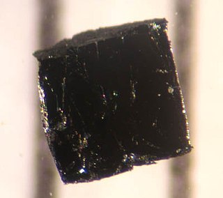Figure: a sample of of Bismuth strontium calcium copper oxide levitating on a magnetic field due to the induced currrents.  Figure: Flying moutnains in the movie *Avatar* are supossed to be made of a high T$_c$ superconducting material that float over on the magnetic poles o the planet. In contrast with the original low temperature superconductors, high T$_c$ ones do not show an isotopic effect, impying that superconductivity does not follow BCS theory. We do not have at present a theoretical description of how superconductivity arises in these kind of materials. There are two possible explanations * The electrons are being paired by some unknown weakly coupled messenger. The leading candidate for that is some perturbation on the magnetic degrees of freedom. * Superconductivity is driven by strong interactions. There is no weakly coupled messenger, but a complete rearrangement of the electron Hilbert space. AdS/CMT stands on the second possibility, using the ability of holography to deal with strongly coupled systems, to try to explain the phase diagram of high T$_c$ superconductors. Such phase diagram is currently under intense study. The emerging picture is very rich, with a variety regions at which the material behave somewhat paradoxically. 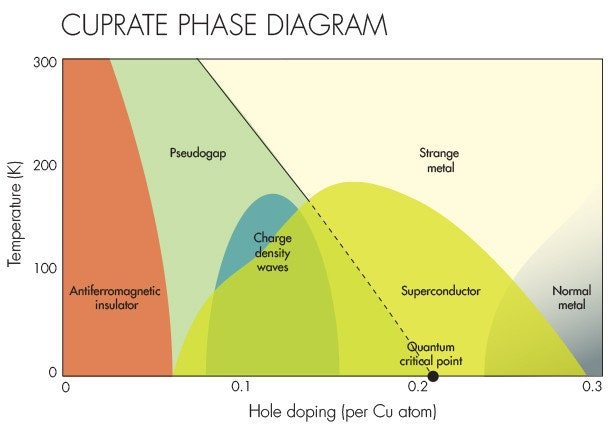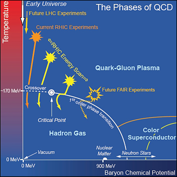The present knowledge can be summarized in the proposal  A point in favour of the hypothesis that the system is driven by strong interactions, is the similarity of the above phase diagram to that of Quantum Chromodynamics, that we know is a strongly interacting theory  However, this is to be taken as a grain of salt, since in both cases we are dealing with proposed phase diagrams in which only some of the points are well known. :::warning :warning: ::: But wait: what does exactly *"strong coupling"* means in a condensed matter setup? Everyday matter is dominated by electromagnetic interactions, that we know are weak at laboratory scales, how can the electrons in a high T$_c$ superconductor be *"strongly interacting"*? The key is on the exchange interaction. Lets assume two single particle states $\Psi(r)$ and $\Phi(r)$. A two electron state is then construced as $|\psi\rangle=\frac1{\sqrt2}\left(\Psi(r_1)\Phi(r_2)-\Psi(r_2)\Phi(r_1)\right)$ The mean value of the interaction energy is given by $\langle\psi|H_{\sf int}|\psi\rangle=\int d^3x_1d^3x_2\,\frac 12{H_{\sf int}}(r_1,r_")\left( |\Psi(r_2)|^2|\Phi(r_1)|^2+|\Psi(r_1)|^2|\Phi(r_2)|^2-\Psi(r_2)^*\Phi(r_1)^*\Psi(r_1)\Phi(r_2) -\Psi(r_1)^*\Phi(r_2)^*\Psi_2\Phi_1 \right)=$ The first two terms represent the classical interaction, while the last two are called exchange integrals. We can consider these energy in an effective Hamiltonian by adding a term $H_{\sf eff}=\dots +\langle\psi|H_{\sf int}|\psi\rangle \hat n_\Phi \hat n_\Psi+\dots$ where $\hat n_\Psi$ and $\hat n_\Phi$ are the operators that gives the number of electrons in states $\Psi$ and $\Phi$ respectively, and they take the values $0,1$. This is an interaction term, since those operators are quadratic in the electron creation and anihillation fields. We see that $\langle\psi|H_{\sf int}|\psi\rangle$ plays the role of the coupling constant. Even if the classical part of the interaction can be small, the exchange part can get much larger, to the point of spoiling the perturbation theory. That's how strong interaction arise effectively in a condense matter system. :::success :white_check_mark: ::: ### Holographic superconductors #### Definition of the model Now, lets try to apply the bottom-up ideas that we developed in the previous lecture to the superconductor context. 1. Symmetry Is is known that most of the electron dynamics in high T$_c$ materials is two-dimensional, that is, it takes place on two dimensional lattice planes inside a three-dimensional crystal with vanishingly small inter-plane coupling.  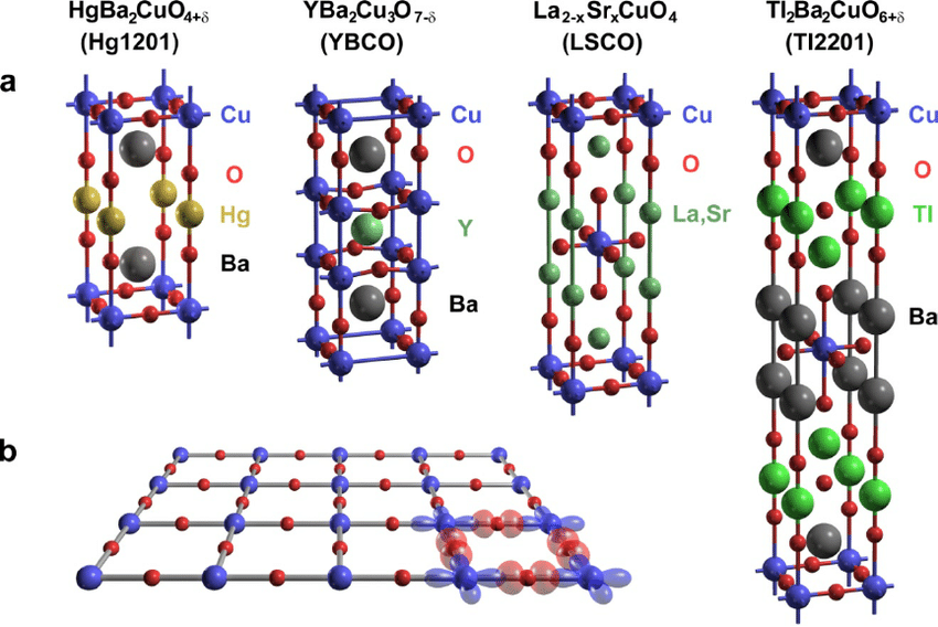Moreover, when temperatures are low enough the lattice is almost invisible for the conduction electrons, whose wavelength is much larger than the lattice parameter. Then the electrons move in an effectively continuous two dimensional space. Depending on the particular lattice, rotational symmetries can still be broken in the aforementioned continuous plane to a discrete subgroup. But in the case of the square lattices, as those shown in the figure, this effect is irrelevant and we can disregard it. :::warning :warning: ::: We can understand the above statement in the language of invariant tensors. The lattice point group is the group of transformations that leave one lattice point invariant (lattice rotations and reflexions). If this group has invariant tensors with indices in the vector representation they can be used to contract derivatives and build invariants to be added to the Lagrangian. In the case of the square lattice, the only invariant tensor with two indices in the vector representation is the Kronecker $\delta_{ij}$, which is invariant not only under the point group, but under the whole $O(2)$. All the tensors in the square lattice which are not invariant under $O(2)$ have more than two indices. So they contribute to terms with more than two derivatives, which are irrelevant in the IR. Then, at low energies the square lattice is rotationally invariant. :::success :white_check_mark: ::: Then the superconductor is described by a two-dimensional continuous rotationally invariant theory, with spacetime point symmetry group $S=O(2)$. In what follows, and in order to get a simpler description, we will enlarge this spacetime point group to $S=SO(2,1)$. Since conduction electrons are conserved, there is a $U(1)$ global symmetry that ensures such conservation. This allows us to write the internal symmetry group as $I=U(1)$ With this, we complete step 1 by constructing an AdS bulk with gravity and a $U(1)$ gauge invariance. 2. Kinematics The electrons on the material are described by an electron field $\chi(x)$, which is an spinor under rotations (or in our simplified version, under Lorentz transformations). This field is charged under the $U(1)$ symmetry. There are many possible composite operators that can be constructed. Of interest to us are the $U(1)$ current $j_\mu=\bar\chi\gamma_\mu\chi$, which is a neutral vector, and the density of Cooper pairs (or *"fermionic condensate"*, which is constructed in Fourier space as proportional to $\chi^\dagger_{-\vec p\uparrow}\chi^\dagger_{\vec p\downarrow}$) and is a charged scalar. Then our field content in the bulk theory will have a fermion $\psi$ (that we will talk about in the next lecture), a vector $A_A$ and a charged scalar $\phi$. We also add the metric, which has an AdS ground state. 3. Dynamics We now need to define have to write an action for the bulk fields. This is very easy, it is just Einstein-Maxwell action with a charged scalar in $2+1$ dimensions $S=\frac1{2\kappa^2}\int d^3x \sqrt{-g}\left(R+\frac 6{L^2}-\frac 14 F_{AB}F^{AB} -|(\partial_A+iqA_A)\phi|^2-{\sf m}^2|\phi|^2\right)$ Finally, we have to solve the resulting field equations with AdS asymptotic conditions, to use the result in the calculation of physical observables. 4. Thermodynamics Since we want to work at finite temperature, we need to include a horizon somewhere in the interior of the geometry. #### Solution ##### Critical temperature The equations of motion of our action read $(\partial_A+iqA_A)^2\phi-m^2\phi=0$ $\partial_A F^{AB}=j^B$ $G_{AB}-\frac3L^2g_{AB}=\kappa^2\, T_{AB}$ Where $T_{AB}$ is given by $T_{AB} = T_{AB}^{\sf EM}+T_{AB}^{\sf Scalar}$ and it includes the electromagnetic and scalar parts $T_{AB}^{\sf EM}=F_{AD} F_B^{~D} - \frac{1}{4} g_{AB} F_{CD} F^{CD}$ $T_{AB}^{\sf Scalar}=(\partial_A-iqA_A)\phi^* (\partial_B+iqA_B)\phi +(\partial_B-iqA_B)\phi^* (\partial_A+iqA_A)\phi - g_{AB} \,m^2 \left(|(\partial_A+iqA_A)\phi|^2+\phi^* \phi\right)$ and the scalar electric current reads $j^A=q\left( \phi \partial_A\phi^*-\phi^* \partial_A\phi \right)+2q^2A_A|\phi|^2$ If the scalar field is nonvanishing in a solution, the $|\phi|^2$ gives a mass to the vector field, implyinig that there is an spontaneous breaking of the $U(1)$ symmetry. To solve the equations, we need an Ansatz $ds^2=L^2\left(-n^2(r)f(r) \,dt^2+\frac 1{f(r)}\,dr^2+r^2(dx^2+dy^2)\right)$ $A=A_0(r)\,dt$ $\phi=\phi(r)$ Plugging the Ansatz into the equations of motion, we get $\phi''+\left(\frac2r+\frac{n'}n+\frac {f'}{f}\right)\phi'+\frac1f\left(\frac{q^2A_0^2}{n^2f}-{\sf m}^2\right)\phi=0$ $A_0''+\left(\frac2r-\frac{n'}n\right)A_0'-\frac{2q^2\phi^2}fA_0=0$ $\frac{2n'}n+r\left(\phi'^2+\left(\frac{q\, n\phi A_0}{L^2f}\right)^2\right)=0$ $\phi'^2+\frac2{r^2}+\frac1{f}\left(\frac {2f'}{r}- 6 +{\sf m}^2\phi^2+\frac{A_0'^2n^2}{L^2}\left(\frac{q^2\, \phi^2}{f}+\frac1{2}\right)\right)=0$ Even if the field $\phi$ is is complex, the equations have real coefficients, implying that a real boundary condition would result in a real solution. We have a total of six derivatives in these equations, so in principle we need six boundary conditions. Since we want AdS asymptotics, our metric functions must satisfy the boundary conditions as $r\to\infty$ $n \approx 1+\dots$ $f\approx r^2\left(1+\dots\right)$ Plugging back into the equations of motion, we can solve for the remaining fields. For the gauge connection we get $A_0=\mu+\dots$ Since the value $\mu$ plays the role of the external source coupled to the boundary electric charge $j_0$, we identify it with the boundary chemical potential. For the scalar we get $\phi=A_+r^{\Delta_+}(1+\dots)+A_-r^{\Delta_-}(1+\dots)$ where $\Delta_\pm=\frac 32\pm\sqrt{\frac {9}{4}-m^2}$ Since we do not want to turn on the condensate by hand, we do not break the $U(1)$ symmetry explicitly. In other words, we impose the boudary condition $A_+=0$ To work at finite temperature, we need to put a horizon at a finite value of the coordinate $r=r_h$ $f(r_h)=0$ at which regularity implies $A_0(r_h)$=0 The temperature is given as usual by Euclideanizing the metric and imposing that there is no conical singularity close to the horizon, where the metric reads $ds_E^2\approx n^2(r_h)f'(r_h)(r-r_h) \,d\tau^2+\frac{dr^2}{f'(r_h)(r-r_h)}+r_h^2(dx^2+dy^2)$ defining $\rho=2\sqrt{(r-r_h)/f'}$ we get $d\rho=dr/\sqrt{f'(r-r_h)}$ or in other words $ds_E^2\approx d\rho^2+\frac14n^2(r_h)f'^2(r_h)\rho^2 d\tau^2+r_h^2(dx^2+dy^2)$ If the length of the circle has to be $2\pi$ times its radious, we get $T=n(r_h)f'(r_h) /4\pi$ An interesting point is that the above equations are invariant under the simultaneous re-scalings of $A_0$ and $r$. This implies that que can replace $A_0\to A_0/\mu$ to put its value at the boudary equal to $1$, while at the same time $r\to r/\mu$, which maps $T\to T/\mu$. In other words, our results will depend on $T$ and $\mu$ through dimesionless combination $T/\mu$, which is consistent with the absense of any other dimensional parameter in the model. Now if $q$ is very large with $qA_0$ and $q\phi$ bounded as well as $\phi'$ and $A'_0$, then the equations simplify to $\phi''+\left(\frac2r+\frac{n'}n+\frac {f'}{f}\right)\phi'+\frac1f\left(\frac{q^2A_0^2}{n^2f}-{\sf m}^2\right)\phi=0$ $A_0''+\left(\frac2r-\frac{n'}n\right)A_0'-\frac{2q^2\phi^2}fA_0=0$ $n'=0$ $\frac2{r^2}+\frac1{f}\left(\frac {2f'}{r}-\frac 6{L^2}\right)=0$ Notice that the metric equations are decoupled and can be solved inmmediately $n=1$ $f=r^2-\frac Mr$ This corresponds to the planar AdS-Schwarzchild black hole solution. This black hole has a horizon at $r_h=M^{1/3}$ and a temperature $T=3M^{1/3}/4\pi$ The remaining equations for $\phi$ and $A_0$ are nontrivially coupled, and have to be solved numerically. This is usually done by shooting: we chose the horizon position $r_h$, which determines the temperature, and integrate the equations of motion to the boundary to check whether the solution satisfy the condition $A_+=0$. If not, we turn on a small $\phi(r_h)$ at the horizon and integrate again. We keep increasing $\phi(r_h)$ until $A_+=0$ is satisfied. The remaining conditions $n\to 1$, $f\to 1$ can be ensured via a change of coordinates. Whenever a non-vanishing value $\phi(r_h)$ is required to have $A_+=0$, this implies that $A_-\neq 0$. In other words, the condensate operator has adquired an expectation value. Since it is a charged operator, the $U(1)$ symmetry has been spontaneously broken. In other words, we have entered the superconducting phase. The results are shown in the figure.  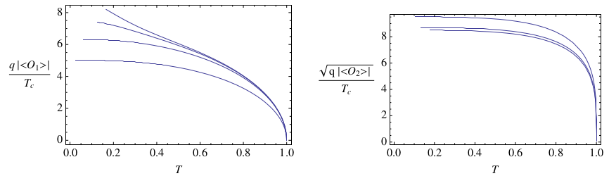Figure: results from the original paper of Hartnoll, Herzog and Horowitz. The mass was chosen as ${\sf m}=-2/L^2$ so both $\Delta_\pm$ give normalizable profiles. The left and right curves correspond to the choice of *"quantization"*, namely wich solution is the expectation value and wich one the external source. As the gravitational coupling is increased by taking smaller $q$'s, the two choices become similar and approach a form which is familiar from high T$_c$ superconductors. ##### Conductivity But of course if we have a superconductor we want to calculate the conductivity. To do that, we need to use the Kubo formula $\sigma_{ij}(\omega, \vec x,\vec y)=\frac{\delta j_i(\omega,\vec x)}{\delta E_j(\omega,\vec y)}=\frac{1}{i\omega}\langle T\{j_i(\omega,\vec x)j_j(\omega,\vec y)\}\rangle$ In our holografic context, that would imply to solve for the field which is the dual of $j_i$, namely the bulk gauge field $A_i$, to obtain its asymptotic behaviour $A_i=a_i^+ A_i^+(r)+a_i^- A_i^-(r)$ and then in Fourier space write $\sigma_{ij}(\omega, \vec x,\vec y)=\frac{ a_i^-}{a_i^+ }$ The equation of motion for a space component of the gauge field $A_i(r)e^{-i\omega t}$ reads $A''_i+\frac{f'}fA'_i+\left(\frac{\omega^2}{f^2}-\frac{2\Phi^2}{f}\right)A_i=0$ We want a causal Green function, namely one in which the response follows the perturbation. This is implicit in the time-ordering of Kubo formula, and in holography it is ensured by imposing causal boundary conditions at the horizon. This is done as follows: the equation of motion close to the the horizon reads $A''_i+\frac{1}{r-r_h}A'_i+ \frac{\omega^2}{(r-r_h)^2}A_i=0$ Changing variables to $u=\log(r-r_h)$ we get $\partial u=(r-r_h)\partial_r$ and $\partial_u^2 A_i+ {\omega^2}A_i=0$ Which admits the solution $A_i\approx \alpha_i^{\sf out} e^{i\omega u}+ \alpha_i^{\sf in} e^{-i \omega u}$. A *causal* setup would imply to impose in-going boundary conditions $\alpha_i^{\sf out}=0$. Now when extending this solution to the boundary, the plane wave form of course get deformed, but the crucial fact that is depends linearly on a single constant $\alpha_i^{\sf in}$ persist. At the boundary, it takes the form with $a_i^+$ and $a_i^-$ written above, but those constant are not intependent but proportional to $\alpha_i^{\sf in}$. The quotient is the independent of $\alpha_i^{\sf in}$ and gives the conductivity.  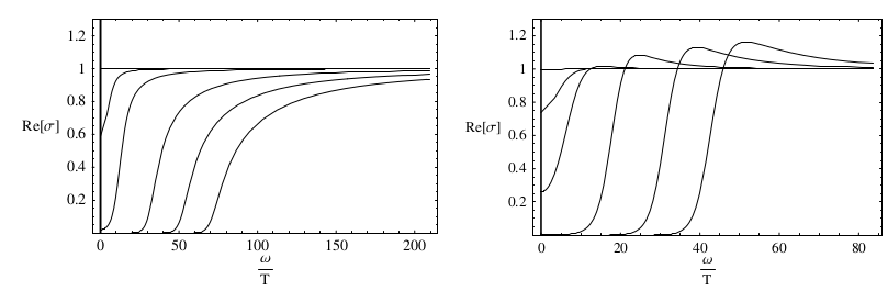Figure: The conductivity as a function of the frequency for different temperatures in the two quantizations, from the same paper as the previous figure. As the temperature is lowered, the curves move to the right and the zero conductivity gap increases. There is a $\delta$ peak at $\omega=0$ due to translational invariance. :::danger :red_circle: ::: ### Sophistications #### Magnetic field We included a gauge field $A_\mu$ in the bulk, to represent the dual of the electric QFT current $j^\mu$. Its time component $A_0$ has a boudary value $\mu$ that we identify with the chemical potential, since it couples as $\mu j^0$. Similarly its spatial part $\vec A$ could have a boudary value $\vec a$ that would couple to the electric current as $\vec a\cdot\vec j$, so it can be identified with the (orbital) magnetic coupling. In particular, if close enough to the boundary $F_{ij}=\partial_iA_j-\partial_jA_i=B\epsilon_{ij}$, we can say that the sample is under a constant magnetic field. This would entail to solve Einstein-Maxwell-Higgs equations with the boundary condition $A_y\to\alpha B\,x$ Writing the equations again $(\partial_A+iqA_A)^2\phi-m^2\phi=0$ $\partial_A F^{AB}=j^B$ $G_{AB}-\frac3L^2g_{AB}=\kappa^2\, T_{AB}$ Where $T_{AB}$ is $T_{AB} = T_{AB}^{\sf EM}+T_{AB}^{\sf Scalar}$ with $T_{AB}^{\sf EM}=F_{AD} F_B^{~D} - \frac{1}{4} g_{AB} F_{CD} F^{CD}$ $T_{AB}^{\sf Scalar}=(\partial_A-iqA_A)\phi^* (\partial_B+iqA_B)\phi +(\partial_B-iqA_B)\phi^* (\partial_A+iqA_A)\phi - g_{AB} \,m^2 \left(|(\partial_A+iqA_A)\phi|^2+\phi^* \phi\right)$ and $j_A$ is $j^A=q\left( \phi \partial_A\phi^*-\phi^* \partial_A\phi \right)+2q^2A_A|\phi|^2$ We notice that if $|\phi|$ is small, the scalar field decouples from the Einstein-Maxwell sector, that can be solved independently. With the Ansatz $ds^2=-n^2(r)f(r) \,dt^2+\frac 1{f(r)}\,dr^2+r^2(dx^2+dy^2)$ $A=A_0(r)\,dt+B\,x\, dy$ We get the magnetic AdS-Reissner-Nordström solution $f(r)=r^2-\frac{1+B^2+(\mu/2)^2}{r}+\frac{B^2+(\mu/2)^2}{r^2}$ $A_0(r)=\mu\left(1-\frac1r\right)$ $A_y= B\, x$ This black hole has a horizon at $r_h=1$, and a temperature given by $T=\frac {1}{4\pi}\left(3-B^2-(\mu/2)^2\right)$ Now we need to solve the equations of $\phi$ in this backgroud. Since the equations necesarily depend on $r$ and $x$, we write an Anzats with the form $\phi=R(r)X(x)$ The equations get separated, obtaining for the $x$ dependence $X''+\left(k^2-q^2B^2x^2\right)\, X=0$ Where $k^2$ is a separation constant. This has normalizable solutions in terms of Hermite functions $H_n$ only when $k^2=2n+1$. Let us concentrate in the $n=0$ solutions, since the higher $n$ have more oscillations, that would naturally result in a higher energy, representing excited states of the condensate. For the $r$ dependence we get $R''+\left(\frac{f'}{f}+\frac2r\right)R'+\frac{2}{f}\left(\frac{q^2A_0^2}{r^2f}+{\sf m}-\frac{qB}{r^2}\right)R=0$ This is the same equation that we got before, but with a correction from the magnetic field. In particular, the same saceling property as before ensures that the result now depends on $T/\mu$ and $B/\mu$. Moreover, it has the same asymtotic behavior $R\approx A_+r^\Delta_++A_-r^\Delta_-$ and we have to solve it with the same boundary conditions. To do that, we first fix $R(r_h)=0$, and move $\mu$ looking for a solution for which $A_+=0$. In case it does not exists, we give to $R(r_h)$ a finite value (since its equation is linear, it doesn't matter which value) and move $\mu$ again, until we find $A_+=0$. This is done for different values of $B$, obtaining a relation $B(\mu)$ (or equivalently $B(T)$) at which the scalar condenses.  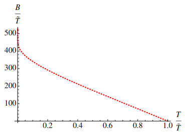Figure: line at which the condensation occurs, from the original paper by Albash and Johnson.  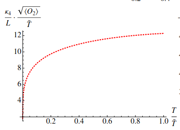Figure: condensate as a function of the temperature, from the original work. This is well bellow the critical temperature, due to the approximation of small $\phi$. #### Doping Up to this point, the chemical potential $\mu$ is not an independent variable, but sets a scale with respect to which the temperature and magnetic field are measured. If we want to have it as an independent parameter, a different scale needs to be set. To do that, one possibility is to include in the bulk kinematics a second gauge field $\tilde A_\mu$, whose boundary value $\tilde A_0\to\tilde\mu$ plays the role of the scale. However, this would represent de bulk dual to a second QFT conserved vector $\tilde j_\mu$, whose physical interpretation is not very clear a priori. We can associate it with a *current of impurities* in the sample. With this somewhat trivial extension, the action reads $S=\frac1{2\kappa^2}\int d^3x \sqrt{-g}\left(R+\frac 6{L^2}-\frac 14 F_{AB}F^{AB}-\frac 14 \tilde F_{AB}\tilde F^{AB} -|(\partial_A+iqA_A+i\tilde q\tilde A_A)\phi|^2-{\sf m}^2|\phi|^2\right)$ Now we would need to write an Ansatz and solve the corresponding equations of motion. Everything would be analogous to the holographic superconductor studied above, with the addition of a gauge field $\tilde A=\tilde A_0(r)dt$ The boundary condition for the new field at the horizon is $\tilde A_0(r_h)=0$ while at the boundary we have $\tilde A_0(r_h)=\tilde\mu+\dots$ This additional scale $\tilde \mu$ would allow us to draw a phase diagram with axes $T/\tilde \mu$ and ${\sf x}=\mu/\tilde\mu$, which represents the doping. Solving the equations with the additional field may look like a complication. However, there is a simple way to do it. After taking the decoupling limit, where $q$ and $\tilde q$ are very large with $qA_0$, $\tilde q\tilde A_0$ and $q\phi$, $\tilde q\phi$ bounded as well as $\phi'$ and $A'_0$, $\tilde A'_0$, they read $\phi''+\left(\frac2r+\frac{n'}n+\frac {f'}{f}\right)\phi'+\frac1f\left(\frac{(qA_0+\tilde q\tilde A_0)^2}{n^2f}-{\sf m}^2\right)\phi=0$ $A_0''+\left(\frac2r-\frac{n'}n\right)A_0'-\frac{2q\phi^2}f(qA_0+\tilde q\tilde A_0)=0$ $\tilde A_0''+\left(\frac2r-\frac{n'}n\right)\tilde A_0'-\frac{2\tilde q\phi^2}f(qA_0+\tilde q\tilde A_0)=0$ $n'=0$ $\frac2{r^2}+\frac1{f}\left(\frac {2f'}{r}-\frac 6{L^2}\right)=0$ The metric is decoupled and can be solved $n=1$ $f=r^2-\frac Mr$ Again the planar AdS-Schwarzchild black hole with a horizon at $r_h=M^{1/3}$ and a temperature $T=3M^{1/3}/4\pi$. The remaining equations can be solved in terms of the combinations $S_0=(qA_0+\tilde q\tilde A_0)/q_{\sf eff}$ and $D_0=\tilde qA_0-q\tilde A_0$, with $q_{\sf eff}=\pm\sqrt{q^2+\tilde q^2}$ as $\phi''+\left(\frac2r+\frac{n'}n+\frac {f'}{f}\right)\phi'+\frac1f\left(\frac{q_{\sf eff}^2S^2_0}{n^2f}-{\sf m}^2\right)\phi=0$ $S_0''+\left(\frac2r-\frac{n'}n\right)S_0'-\frac{2q_{\sf eff}^2\phi^2}fS_0=0$ $D_0''+\left(\frac2r-\frac{n'}n\right)D_0'=0$ The combination $D_0$ is completely decoupled and can be set to zero, while the remaining equations represent the undopped superconductor that we already solved. Those equations resulted in a critical temperature defined as $T_c$ that, due to the aforementioned scaling symmetry, is proportional to $\mu_S$ (that is the boudary value of $S_0$). 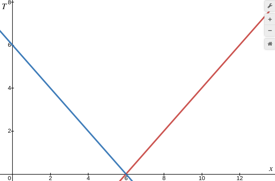We can write $T_c=\beta \mu_S$ This can be rewritten in terms of the original fields as $T_c= \frac \beta {q_{\sf eff}}(q\mu+\tilde q\tilde \mu)$ Defining the doping variable as ${\sf x}=\mu/\tilde \mu$ we get $T_c=\frac {\beta \tilde \mu} {q_{\sf eff}}(q\,{\sf x}+\tilde q)$ This results in the phase diagram  Figure: phase diagram for $q=1, \tilde q=3$ and $\beta\mu/e_{\sf eff}=1$ As we see, the results are not very good but promising. 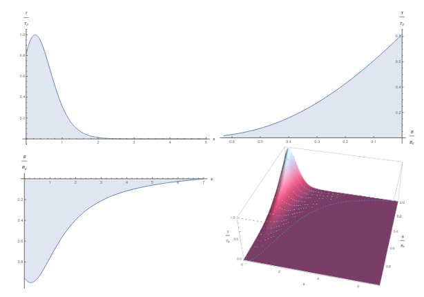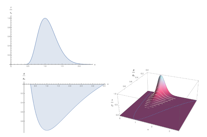This is due to the probe aproximation we used, in the magnetic case, where the gravitational backreaction of the electromagnetic field is not neglected, the results are much better  Figure: the phase diagram of a holographic superconductor under a magnetic field, for certain values of $q$ and $\tilde q$ from Correa *et al.*  Figure: the phase diagram of a holographic superconductor under a magnetic field, for certain values of $q$ and $\tilde q$ from Correa *et al.*  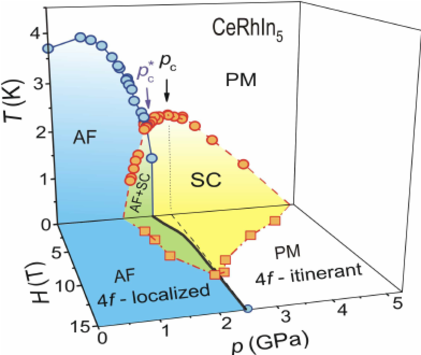Figure: Experimental points and propose pahse diagram for the compound CeRhIn$_5$, from *Trends in heavy fermion matter* by Flouquet *et. al.* #### $p$-wave superconductors In the above discussion, we assumed that electrons in Cooper pairs are bounded in a spin zero state, the condensate operator being proportional to $\chi_{-\vec p\uparrow}^\dagger\chi_{-\vec p\downarrow}^\dagger$. This resulted in a charged scalar QFT operator, dual to a bulk charged scalar field. But there is another possibility, that of the electrons in the pair forming a triplet $(\chi_{-\vec p\downarrow}^\dagger\chi_{-\vec p\downarrow}^\dagger,\chi_{-\vec p\uparrow}^\dagger\chi_{-\vec p\downarrow}^\dagger,\chi_{-\vec p\uparrow}^\dagger\chi_{-\vec p\uparrow}^\dagger)$. We will assume that it is a vector under both spacetime point symmetry and internal spin symmetry, independently. This defines a charged vector QFT operator, and the dual field would have to be described by a charged vector field. A charged vector field in the bulk cab be included in the context of a non-Abelian gauge theory. The non-Abelian gauge field $A_\mu^a$ transforms as a vector under both internal symmetries and spacetime rotations, independently. It is charged under some $U(1)$ subgroup of the non-Abelian gauge group. So it contains at the same time the dual to both the (now vector-like) condensate, and the particle current. We write the Lagrangian $L=\frac1{2\kappa^2}\left(R+\frac 6{L^2}\right)-\frac{1}{4e^2}F_{AB}^aF^{a\,AB}$ We have to solve the equations of motion with the Ansatz $ds^2=L^{2}\left(-f(r)n^2(r)dt^2+\frac{dr^2}{f}+\frac{dx^2}{g(r)}+g(r)dy^2\right)$ $A=A_0(r)\tau_0\,dt+W(r)\tau_1 \,dx$ Notice that it is an anisotropic Ansatz, and if the condensate $W$ is turned on, then rotational invariance is broken and the $g\neq 0$.  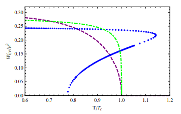Figure: the condensate as a function of the temperature, from Giordano *et. 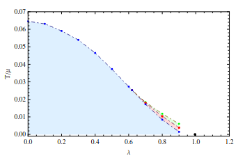al.*  Figure: the phase diagram in the plane temperature *vs.* coupling $\lambda=\kappa/Le$, from Giordano *et. al.* #### Coleman-Mermin-Wagner theorem The famous Coleman-Mermin-Wagner theorem states that *there are no local systems in two dimensions that exhibit spontaneous breaking of a continuous global symmetry at finite temperature*. But we just found one!.. The spontaneous breaking of a continuous global symmetry implies that there is some operator ${\cal O}$ in the QFT that is charged under the symmetry and adquires an expectation value on the ground state. In the superconductor that operator is given by the Cooper pair condensate. An important point to be considered is that the fluctuations of the expectation value $\sigma^ 2=\langle{(\cal O}-\langle{\cal O}\rangle)^2\rangle=\langle{\cal O}^2\rangle-\langle{\cal O}\rangle^2$ are small. regularizing with a point spliting we get $\sigma^2=\lim_{x\to x'}\left(\langle{\cal O}(x){\cal O}(x')\rangle-\langle{\cal O}(x)\rangle \langle{\cal O}(x')\rangle\right)=$ Defining the fluctuation operator as $\delta {\cal O}={\cal O}-\langle{\cal O}\rangle$ we can write $\sigma^2=\lim_{x\to x'}\langle\delta {\cal O}(x)\delta {\cal O}(x')\rangle$ At low enough energies, these fluctuations are dominated by the massless modes. In the case of a state that breaks spontaneously a continuous symmetry, these are the Nambu-Goldstone bosons $\sigma^2\sim\lim_{x\to x'}\langle\pi(x)\pi(x')\rangle$ The expectation value on the right hand side is nothing but the propagator of a scalar field. It can be obtained by writing an effective Lagrangian for the Nambu-Goldstone modes, and then performing a straightforward QFT calculation. In $1+1$ dimensions, or in $2+1$ dimension at finite temperature, it reads $\sigma^2\sim\lim_{x\to x'}\log(x-x')$ This is naturally UV divergent, what could have been expected and is assumed to be regularized, but it is also IR divergent. The natural IR cutoff is given by the inverse of the size of the sample, implying that for large enough samples $\sigma^2$ diverges. How are holographic superconductors evading the consequencies of the theorem? We are working in a $3+1$ dimensional space, in which the scalar field propagator do not have IR divergences. Moreover, the bulk symmetries are gauged, implying that there are no Nambu-Goldstone bosons. However, if holographic duality works, there have to be some analogous to Coleman-Merming-Wagner theorem for gauge symmetries in $3+1$ asymtotically AdS dimensions. Moreover, since we have already proved that spontaneous symmetry breaking occurs at the classical level, the effect has to be quantum, showing up at one loop. One way to include one loop effect is adding to the classical bulk Lagrangian higher order terms arising from loop corrections. This is straitforward for the bulk scalar $\phi$ and gauge field $A_A$, but in the case of the gravitational action is non-trivial. Indeed, higher order corrections to Einstein-Hilbert action in $3+1$ dimensions are tricky, since they potentially trigger ghost-like instabilitites. A particularly healthy action that was recentely studied in the literature is Einsteinian cubic gravity. Is is given by $S_{\sf Gravity} = \frac{1}{2\kappa^2} \int d^4x \, \sqrt{-g} \left( R +\frac{6}{L^2} - %2 \beta \frac{\beta}{54} (\mathcal{P} - 8 \mathcal{C}) \right)$ where $\mathcal{P} = 8 R_{a}{}^{b} R_{b}{}^{c} R_{c}{}^{a} - 12 R^{ac} R^{bd} R_{abcd} + 12 R_{a}{}^{c}{}_{b}{}^{d} R_{c}{}^{e}{}_{d}{}^{f} R_{e}{}^{a}{}_{f}{}^{b} + R_{ab}{}^{cd} R_{cd}{}^{ef} R_{ef}{}^{ab} ~$ $\mathcal{C} = R_{abcd} {R}^{abc}_{~~~e} {R}^{de} - \frac{1}{4} R_{abcd}R^{abcd}R - 2 R_{abcd}R^{ac}R^{bd} + \frac{1}{2} {R}_a^b{~b} {R}_b^{~a} R ~$ We can couple it to the scalar and gauge field parts, and try to solve the holographic superconductor with those higher curvature corrections. The EOM are $f n r^3 \Big[ 2r n^2 \left( 6 \frac{r}{L^2} - m^2r \phi ^2-2f' \right) -2f n^2 \left( r^2 \phi '^2 + 2 \right) -r^2 A_0'^2 \Big] -2 q^2 r^5 n \phi ^2 A_0 ^2$ $+ \frac 2{27} \,\beta \bigg\lbrace \phantom{2^{2^2}}\!\!\!\!\!\!\! 24 f^2 n^3 f' (rf' - f ) - 24 f^4 n' \big(2(r^2 n'^2-n^2)+r n n' \big)+$ $+6rff'n'\Big[ 8 f n^2 (rf'-2f)- r^2 n f'(5 f n'+2 n f') +4rf^2n'(4 n + r n' ) \Big]+$ $+6rnf^2f'' \Big[ 4 f\big( - r n^2 f' +( n^2 + r nn' - r^2 n'^2 ) \big)+ r^2 n^2 f'' \Big]+$ $+12rf^2nn'' \Big[ 2f^2(3 r n' - n)+rf' \big( n (2 f - r f') -3 r n'f \big) + r^2 n ff'' \Big]+$ $+3r^2n^2 f^3f^{(3)} \big( 4 (r n'- n) + 2 r f^2 n f' \big)\bigg\rbrace = 0$ $nr^3 \Big( 2 f^2 n n'-r f^2 n^2 \phi '^2-q^2 r \phi ^2 A_0 ^2 \Big)$ $+\frac 2{27} \,\beta \bigg\lbrace 3n' \Big[ 4 n^2f^2 f' (r f' -2 f ) +f^2 n' \big( 4 f^2 (n -2 r n') +3 r^2 f' ( 2 f n' -n f') \big) \Big]$ $+ 3 nf^2 n'f'' \Big[ nr(8 f-5 rf')-6 r^2 f n' \Big]$ $+3f^2n'' \Big[ 2n' f \big( 2nr (f -3 r f')+ r^2 f n' \big) +n^2 \big( 2f ( 4 r f' - f ) -3 r^2 F'^2 \big) \Big]$ $-3r^2nf^3 n'' \big( 2f n'' + n f'' \big)- 3rnf^3 n^{(3)} \big( 2 f(r n' - n)+ r n f' \big) \bigg\rbrace = 0$ Even if they look awful, results can be found numerically, obtaining  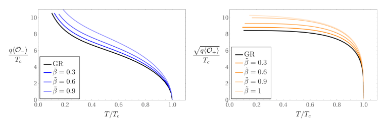Figure: condensate value for different values of the higher curvature coupling  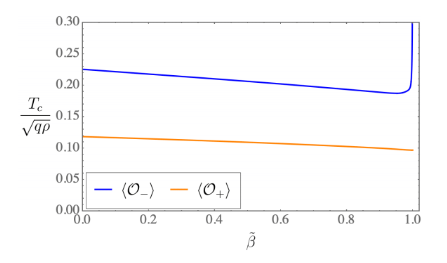Figure: critical temperature as a function of the higher curvature coupling We see that the condensation becomes more difficult as the higher curvature cupling is increasing. But the expected effect was the complete dissapeareance of the condensate. This failure could have been anticipated from the beginning: highe curvature corrections affect the UV behaviour of a field theory, while Coleman-Mermin-Wagner theorem is based on an IR divergence. The correct approach would be calculate the fluctuation of the scalar field up to one loop in the bulk fields, looking for a contribution that diverges on the IR. This was done by Anninos *et. al.* --- ## Lecture 3: holographic metals :::success :white_check_mark: :::  Figure: no, not that metal  Figure: this metal ### Introduction to Fermi liquids A metallic state is describe by Landau's theory for the Fermi liquid. It can be uderstood as a deformation of the Fermi gas, as follows. We describe a Fermi gas starting with the free Dirac Lagrangian $\cal L=\bar\chi(i\partial\!\!\!/-m)\chi$ we obtain it single particle states by writing Dirac equation $(i\partial\!\!\!/-m)\chi=0$ Fourier trasforming $(\omega\gamma^0-\vec k\cdot\vec\gamma-m)\chi=0$ Multiplying by $\gamma^0$ it becomes an eigenvalue equation that results in the values of $\omega=\pm\sqrt{ k^2+m^2}$. The negative energy particle staet are reinterpreted as positive energy particle states, resulting in the dispersion relation $\omega=\sqrt{ k^2+m^2}$. To construct the Fermi gas ground state, these single particle states are then filled one by one until we exhaust the available particles, in ohter words, until the energy reaches the chemical potential $\omega=e\mu\equiv \mu_e$. This defines the Fermi energy as $\omega_F=\mu$ and a Fermi momentum $|k_F|=\sqrt{ \mu^2_e-m^2}$. The Fermi surface is then the locus in momentum space where $|\vec k|=k_F$ The excitations of the ground state are defined by removing one particle from a single particle state bellow the Fermi energy (*i.e.* inside the Fermi surface), and plugging it in some single particle state above the Fermi energy (*i.e.* outside the Fermi surface). This can be described by a field theory for the excitations, which is simply constructed as a free spinor field $\chi(x)$ with Lagrangian $\cal L=\bar\chi(i\partial\!\!\!/-m)\chi-\mu_e \chi^\dagger\chi$ This is the usual Dirac lagrangian to which we added a chemical potential as the external source for the number of particles. The resulting EOM read $(i\partial\!\!\!/-\mu_e\gamma^0 -m)\chi=0$ In Fourier space we get $((\omega-\mu_e)\gamma^0-\vec k \cdot\vec\gamma -m)\chi=0$ The left hand side has eigenvectors $\chi_\pm$ allowing us to write $(\omega-\mu_e\pm\sqrt{k^2+m^2})\chi_\pm=0$ Defining the particle wavefunction as $\chi_P=\chi_-$ and the hole one as $\chi_H(\omega) =\chi_+(-\omega)$, we get the dispersion relation for particles and holes as $\omega=\epsilon(k)$ with $\epsilon(k)=\mu_e+\sqrt{k^2+m^2}$. The retarded Green function for these excitations read $G=\lim_{\eta\to 0}\frac1{\omega-\epsilon (k) +i\eta}$ This implies $\Re(G)=\lim_{\eta\to 0}\frac{\omega-\epsilon (k)}{(\omega-\epsilon (k))^2 +\eta^2}=\frac1{\omega-\epsilon (k)}$ $\Im(G)=\lim_{\eta\to 0}\frac{-\eta}{(\omega-\epsilon (k))^2 +\eta^2}=-\pi\,\delta (\omega-\epsilon (k))$ The moral of this is that the Green function of a Fermi gas has a pole at the Fermi surface in its real part, and a delta peak in its imaginary part. Now the Fermi liquid is defined by introducing perturbative interactions among the ground state excitations of the Fermi gas. There interaction excitations are now called *quasiparticles* and *quasiholes*. When interations are present, energy gets renormalized by the quasiparticle self energy loops $\Sigma(k)$ as $\omega=\epsilon(k)+\Sigma(k,\omega)$. Writing $\Sigma(k,\omega)=\delta\epsilon(k,\omega)+i\Gamma(k,\omega)$ we obtain $\omega=\epsilon(k)+\delta\epsilon(k,\omega)+i\Gamma(k,\omega)$. Notice than the effect of $\Sigma(k,\omega)$ is to renormalize the dispersion relation and adding an imaginary part to it. This results in a time evolution of the excitation with a factor $e^{-\Gamma(k,\omega)t}$, so it is fair to say that $\tau=1/\Gamma(k,\omega)$ is the mean lifetime of an excitation. The resulting Green function is also modified by the quasiparticle self energy, as $G=\lim_{\eta\to 0}\frac1{\omega-\epsilon (k) +i\eta-\Sigma(k,\omega)}$ This implies $\Re(G)=\frac{\omega-\epsilon (k)-\delta\epsilon(k,\omega)}{(\omega-\epsilon (k)-\delta\epsilon(k,\omega))^2 +|\Gamma(k,\omega)|^2}$ $\Im(G)=-\frac{\Gamma(k,\omega)}{(\omega-\epsilon (k)-\delta\epsilon(k,\omega))^2 +|\Gamma(k,\omega)|^2}$ We see that the effect of $\Sigma(k,\omega)$ is to shift and thicken the $\delta$-like peak at the Fermi surface. In other words, the Fermi surface has moved and got smoother. In order for the description to be consistent, low energy excitations has to be long lived. In other words, we need $\Sigma(k,\omega)\to0$ close enough to the fermi surface. Notice that it need to go to zero faster than $\omega-\epsilon (k)-\delta\epsilon(k,\omega)$, in order to recover the $\delta$-like peak in this limit. ### Holographic metals In order to construct and holographic dual for the fermionic derees of freedom of our superconductor, we need to consider the field $\psi$ that we set to zero up to now. Including it in the action $S=\frac1{2\kappa^2}\int d^3x \sqrt{-g}\left(R+\frac 6{L^2}-\frac 14 F_{AB}F^{AB} -|(\partial_A+iqA_A)\phi|^2-{\sf m}^2|\phi|^2+\bar \psi(i\partial\!\!\!/+\frac14\omega_{ab}\!\!\!\!\!\!\!\!/\ \ \ \,\Gamma^{ab}-eA\!\!\!/-m)\psi\right)$ We get the equations of motion $(i\partial\!\!\!/+\frac14\omega_{ab}\!\!\!\!\!\!\!\!/\ \ \ \,\Gamma^{ab}-eA\!\!\!/-m)\psi=0$ $(\partial_A+iqA_A)^2\phi-{\sf m}^2\phi=0$ $\partial_A F^{AB}=j^B$ $G_{AB}-\frac3L^2g_{AB}=\kappa^2\, T_{AB}$ Where $T_{AB}$ is given by $T_{AB} = T_{AB}^{\sf EM}+T_{AB}^{\sf Scalar}+T_{AB}^{\sf Matter}$ and it includes the electromagnetic, scalar and matter parts $T_{AB}^{\sf EM}=F_{AD} F_B^{~D} - \frac{1}{4} g_{AB} F_{CD} F^{CD}$ $T_{AB}^{\sf Scalar}=(\partial_A-iqA_A)\phi^* (\partial_B+iqA_B)\phi +(\partial_B-iqA_B)\phi^* (\partial_A+iqA_A)\phi - g_{AB} \,m^2 \left(|(\partial_A+iqA_A)\phi|^2+\phi^* \phi\right)$ $T_{AB}^{\sf Matter}=$ we'll see later and the electric current reads $j^A_{\sf Scalar}+j^A_{\sf Matter}$ where $j^A_{\sf Scalar}=q\left( \phi \partial_A\phi^*-\phi^* \partial_A\phi \right)+2q^2A_A|\phi|^2$ $j^A_{\sf Matter}=$ we'll see later Here we chose a basis for the bulk gamma matrices as $\Gamma^r=\left(\begin{array}{cc}1&0\\0&-1\end{array}\right)$ $\Gamma^r=\left(\begin{array}{cc}0&\gamma^\mu\\\gamma^\mu&0\end{array}\right)$ Where $\gamma^\mu=(i\sigma_2,\sigma_1,\sigma_3)$ are the boundary gamma matrices. Since we are interested in the strange metal region of the phase diagram, we have no fermionic condensate so we set $\phi=0$. This leads us to the Ansatz $ds^2=L^2\left(-n^2(r)f(r) \,dt^2+\frac 1{f(r)}\,dr^2+r^2(dx^2+dy^2)\right)$ $A=A_0(r)\,dt$ $\psi=L^2r\sqrt{n}\,e^{i(\vec k\cdot\vec x-\omega t)}\left(\begin{array}{c}\psi_{+u}\\\psi_{+d}\\\psi_{-u}\\\psi_{-d}\end{array}\right)$ We are interested in perturbations of the ground state, so the field $\psi$ is small. This implies that anything quadratic in $\psi$ can be consistently disregarded in the equations of motion. This in particular affects the fermioninc part of the current $j^A_{\sf Matter}$ and that of the energy momentum tensor $T_{AB}^{\sf Matter}$. With these considerations, when we plug the Ansatz into the equations of motion we get $\psi_{\pm u}' \mp\frac m{\sqrt f} \psi_{\pm u}=\mp \frac i{{r}\sqrt{f}}\left(k_x-\frac r{n\sqrt f}(\omega+A_0)\right)\psi_{\mp d}$ $\psi_{\mp d}' \pm\frac m{\sqrt f} \psi_{\mp d}=\pm \frac i{{r}\sqrt{f}}\left(k_x-\frac r{n\sqrt f}(\omega+A_0)\right)\psi_{\pm u}$ $A_0''+\left(\frac2r-\frac{n'}n\right)A_0'=0$ $\frac{2n'}n=0$ $\frac2{r^2}+\frac1{f}\left(\frac {2f'}{r}- 6 +\frac{A_0'^2n^2}{2L^2} \right)=0$ where we used rotational invariance to put $\vec k=(k_x,0)$. The equations for $A_0$, $n$ and $f$ are completely decoupled from the fermion. When solving them with the same boudary conditions as before, we obtain the Reissner-Nordström solution $f(r)=r^2-\frac{1+(\mu/2)^2}{r}+\frac{(\mu/2)^2}{r^2}$ $A_0(r)=\mu\left(1-\frac1r\right)$ This black hole has a horizon at $r_h=1$, and a temperature given by $T=\frac {1}{4\pi}\left(3-(\mu/2)^2\right)$ Close to the boundary the equations of motion give the behaviour $\psi_{+}=A r^m+\frac {ik\!\!/}{2m+1}D r^{-m-1}$ $\psi_{-}=\frac {ik\!\!/}{2m+1}A r^m+D r^{-m-1}$ where $\phi_\pm$ are two-component spinors, and so are $A$ and $D$. When we expand close to the horizon and impose in-going boundary conditions, the two spinors $A$ and $B$ become linearly related $D={\cal S}A$. 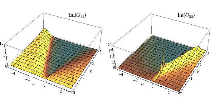The correlator is then given by $G=-i{\cal S}\gamma^0=\lim_{r\to0}r^{-2m}\left(\begin{array}{cc}\frac{i\psi_{-u}}{\psi_{+d}}&0\\0&-\frac{i\psi_{-d}}{\psi_{+u}}\end{array}\right)$ With this, we can calculate the Green function  Figure: the imaginary part of the two components of the Green function, from the original paper by Liu, McGreevy & Vegh. We may want to introduce backreaction into this setup. This is subtle, because of Pauli exclusion principle: a classical state with fermions *is not* the classical solution of Dirac equation. Indeed, in the case of a scalar, the classical limit satisfies $\langle T_{AB}(\phi)\rangle\approx T_{AB}(\langle \phi\rangle)$. But, due to the filling o the one particle states up to the fermi surface, we have that for a fermion $\langle T_{AB}(\psi)\rangle\approx \!\!\!\!\!\!/\ \ T_{AB}(\langle \psi\rangle)$. The correct way to describe the classical ground state of many fermions is via a fluid. Representing it as a perfect fluid with four-velocity $u_A$ satisfying $u^Au_A=-1$, we can write for the energy momentum tensor $T_{AB}^{\sf Matter}=(p+\rho)u_Au_B+pg_{AB}$ and for the electric current $j^A=\sigma u_A$ where $p$ is the pressure, $\rho$ is the energy density, and $\sigma$ the particle density. We need an expression for these quantities, that we can calculate in the Thomas-Fermi approximation, assuming that the wavelength of the fermionic fluid particles is small as compared with the scales relevant to the geometry $\sigma=\beta\int_m^{p_F} d^3p$ $\rho=\beta\int_m^{p_F} d^3p\sqrt{p^2+m^2}$ $-p=\rho-\mu_e\sigma$ In these expressions, $p_F$ is obtained as the value of $p$ at which the energy equals the local chemical potential $\sqrt{p_F^2+m^2}=A_0n\sqrt f$. After we make the Ansatz for the fluid velocity $u^A=(u^0(r),0,0,0)$, obtaining $u^0=1/n\sqrt{f}$, the resulting equations of motion read $r^3\left( \frac {2n'}{n}-\frac{4f}r\right)-\frac {A_0\sigma}{n \sqrt f}=0$ ${f'}+ \frac f{r}+ \frac{{2f}n'}{n}+\frac {r A_0'^2}{2n^2 }-\frac 1{ r^3}(3+p)=0$ $fr^2(r^2A_0')'-\frac{\sigma}{n\sqrt f}\left(\frac 1{2 } rA_0A_0h'+n^2f\right)=0$ where we have re-scaled the variables $p$, $\sigma$, $\rho$ and $A_0$ to eliminate $e$, $\kappa$ and $L$ factors. We solve these equations at small $r$, obtaining a Lifshitz solution $n=r^{z+1}$ $f=f_{IR}(z) r^{-2}$ $A_0=A_{IR}(z) r^z$ The explicit dependence on $z$ of the coefficients $f_{IR}$ and $A_{IR}$, as well as the functional relation between $z$ and $m,\beta$, is obtained by plugging the above Lifshitz form into the equations of motion. Now we perturb this solution, searching for a perturbation that grows towards the UV $r\to\infty$ and dies towars the IR $r\to0$. 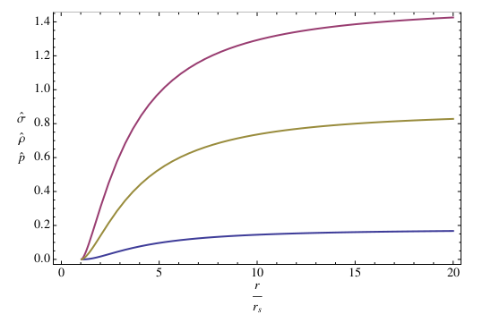The boundary of the star is reached when the local chemical potential becomes smaller than the mass $A_0n\sqrt f=m$  Figure: profile for the star quatities from the original paper by Hartnoll & Tavanfar (the radil varaible is inverted wrt the one we use in the present lectures) :::warning :warning: ::: If we want to evaluate the on shell action, in order to use the holographic path integral formula, we would need an action that provides the fluid equations. This is done with the Shutz action ${\cal L}=-\rho(\sigma)+\sigma u^A(\partial_A\varphi+A_A)+\lambda(u^Au_A+1)$ Variation of this action gives the equations $u^Au_A=-1$ $\partial_A(\sigma u^A)=0$ $\rho'(\sigma)=\mu=u^A(\partial_A\varphi+A_A)$ $\sigma(\partial_A\varphi+A_A)+2\lambda u^A=0$ Multiplying the later by $u^A$ and using the first $\lambda=\sigma\mu/2$ Now replacing again in the last $u^A=-(\partial_A\varphi+A_A)/\mu$ Moreover, varying with respect to the gauge field $A_A$ we obtain the right form of the electric current, while doing so with respect to the metric we obtain the energy-momentum tensor. :::success :white_check_mark: ::: We can now calculate the conductivity, by turning on a perturbative gauge component in the $x$ direction. The backreaction excites perturbations on the metric and the fluid four-velocity, and we get $\sigma A_x+(p+\rho)u_x=0$ $r^2g_{tx}'-2rg_{tx}-2A_0'A_x=0$ $(r^2A')'_x-\left(\frac {f'}f+\frac {n'}{n}\right)A_x+\frac{A_0'}{n^2f}\left( r^2g_{tx}'- 2rg_{tx}\right)+\frac{\sigma}{r^2f} u_x+\frac {\omega^2}{r^2n^2f^2}A_x=0$ Eliminating $g_{tx}$ and $u_x$ we have $r^2(r^2A_x)+r^2\left(\frac{f'}f+\frac{n'}{n}\right)A_x'+\left(\frac{\omega^2}{n^2f^2}-\frac{\sigma^2}{f(p+\rho)}-\frac{2A_0'^2}{n^2f}\right)A_x=0$ This equation is solved with causal boundary conditions at $r\to0$ to obtain the conductivity in the standard way  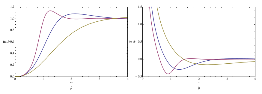Figure: the conductivity for different values of $\beta$ and $m$, from the original paper :::danger :red_circle: ::: ### Sophistications #### Temperature Introducing finite temperature in the backreacting setup is not complicated, we just change teh boundary condition from a Lifshitz scaling in $r\to 0$ to black hole conditions of the form $f(r_h)=0$ $A_0(r_h)=0$ Since we start with vanishing $A_0$, the local chemical potential is zero just outside the horizon, and starts to grow as we get away from it. When it reaches $m$ the fluid appears, and persist for larger $r$ until the chemical potential gets bellow $m$ again. Thus a *floating cloud* of fluid appears just above the horizon, in equilibrium between the gravitational repulsion from the AdS boudary and the electronstatic repulsion from the black hole. As the temperature is rised, the clud gets smaller, until a critical temperature at which is dissappears.  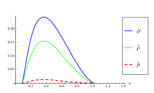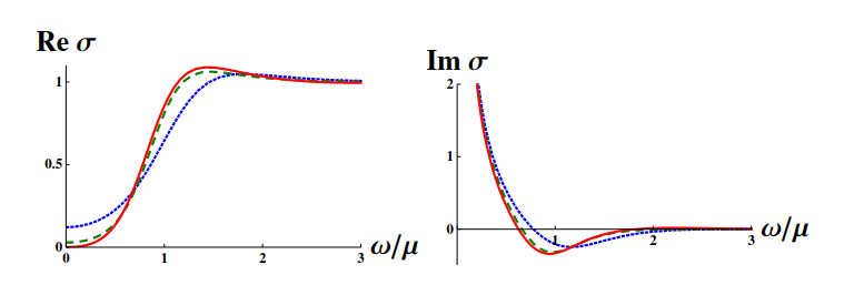Figure: profile of the electron star functions at finite temperature, from the original work of Giangreco *et al.*  Figure: conductivity at finite temperature, from the original work of Giangreco *et al.* #### Doping When we introduce doping by adding a second gauge field, there is again a transformation that maps the problem into the undoped one. For the case of the non-backreactin metal, the quasiparticle lifetime depends on $\omega$ in a way that includes the doping. 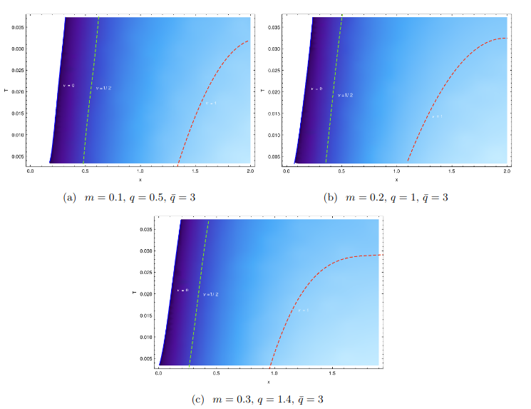This implies that the region in which the system obbeys Landau's theory can be identified in phase space  Figure: region where stable quasiparticles exist, and where the systems obbeys Landau's theory. A similar mapping can be done in the backreacting case. #### Turning on the superconductor The metallic degrees of freedom still exist when we are in the superconducting phase, so questions such that the existence of a Fermi survace and that of stable quasiparticles can still be formulated. For example, in the case of a $p$-wave superdoncuctor, rotational invariance is broken and the Fermi surface should reflect that. Moreover, the breaking of rotational invariance can give place to the appeareance of*Fermi pockets* and *Fermi arcs* afeature that has been observed in high T$_c$ superconductors.  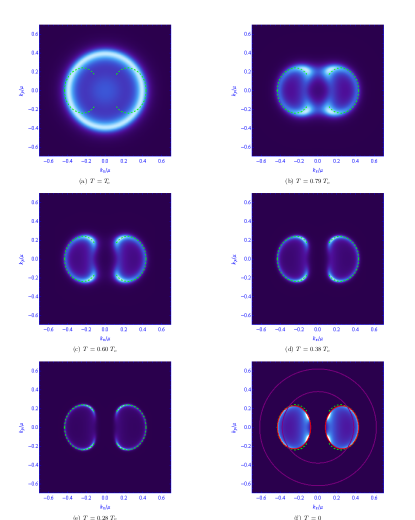Figure: we see the anisotropy showing up as the superconducting phase condenses, and later we see the appeareance of Fermi arcs in the spectral function. ## Fin  $\phantom{\frac12}$ $\phantom{\frac12}$ $\phantom{\frac12}$ $\phantom{\frac12}$ $\phantom{\frac12}$ $\phantom{\frac12}$ $\phantom{\frac12}$ $\phantom{\frac12}$ $\phantom{\frac12}$